Path analysis and Structural Equation Modeling (SEM) allow us to test hypotheses about the direct and indirect effects among observed and latent variables, but they do so in slightly different ways.
Path analysis is a precursor to SEM and is used to assess the direct and indirect relationships between measured variables. It’s really a specialised case of multiple regression that allows for the exploration of models with multiple dependent variables.
Path analysis is represented through diagrams that illustrate the causal relationships between variables, with arrows indicating the direction of the relationship.
So, path analysis:
Focuses on observed variables.
Deals with direct and indirect effects but does not include latent variables.
Uses regressioncoefficients to estimate the strength of the relationships.
SEM extends path analysis by including latent variables (unobserved variables that are inferred from observed variables) in addition to the observed variables. This makes SEM a more powerful and flexible technique than path analysis. SEM encompasses a broader array of models, including confirmatory factor analysis, path analysis, and others, allowing for the analysis of complex relationships between observed and latent variables.
So, SEM:
Incorporates both observed and latent variables.
Can model multiple levels of relationships simultaneously, including mediation and moderation effects.
Uses covariance among variables to estimate model parameters, creating a more complex view of variable interrelations.
38.2 Path analysis: demonstration
38.2.1 Step One: Create a dataset
Show code for dataset creation
rm(list=ls())# Load necessary librarylibrary(tidyverse)# Set seed for reproducibilityset.seed(123)# Generate synthetic datasetn <-200# Number of observations# Independent VariablesPossessionTime <-round(rnorm(n, mean=30, sd=5),2)Tackles <-round(rpois(n, lambda=20),0)SuccessfulPasses <-round(rpois(n, lambda=150),0)TerritorialGain <-round(rnorm(n, mean=1000, sd=200),2)PenaltiesConceded <-round(rpois(n, lambda=10),0)# Generating PerformanceScore with associationsPerformanceScore <-round(50+ (PossessionTime *0.5) + (SuccessfulPasses *0.05) - (PenaltiesConceded *1) +rnorm(n, mean=0, sd=5),2)df <-tibble(PossessionTime, Tackles, SuccessfulPasses, TerritorialGain, PenaltiesConceded, PerformanceScore)# Print out the first few rows to checkhead(df)
The dataset contains data for 200 rugby games, and has been reduced to the following variables:
PossessionTime - Time in possession of the ball (in minutes).
Tackles - Number of tackles made.
SuccessfulPasses - Number of successful passes.
TerritorialGain - Total territorial gain (in meters).
PenaltiesConceded - Number of penalties conceded.
PerformanceScore - Game evaluation by three independent coaches.
38.2.2 Step Two: Exploratory Data Analysis (EDA)
The first step in Path Analysis is to define our model.
In this instance, our analysis is based on exploring the interactions between our independent variables (IVs) and the dependent variable (DV), which we have determined will be PerformanceScore.
We’ll start, as always, by conducting some EDA on the data. After some descriptive statistics, we’ll concentrate on exploring the relationships between the different variables, as this will be the focus of our subsequent Path Analysis.
 PossessionTime     Tackles   SuccessfulPasses TerritorialGain
 Min.   :18.45   Min.   :10   Min.   :112.0    Min.   : 498.4
 1st Qu.:26.87   1st Qu.:17   1st Qu.:142.0    1st Qu.: 879.2
 Median :29.70   Median :20   Median :150.5    Median :1028.6
 Mean   :29.96   Mean   :20   Mean   :150.0    Mean   :1016.5
 3rd Qu.:32.84   3rd Qu.:23   3rd Qu.:159.0    3rd Qu.:1157.9
 Max.   :46.21   Max.   :35   Max.   :187.0    Max.   :1538.3
 PenaltiesConceded PerformanceScore
 Min.   : 3.00     Min.   :48.66
 1st Qu.: 8.00     1st Qu.:58.83
 Median :10.00     Median :62.44
 Mean   : 9.93     Mean   :62.48
 3rd Qu.:12.00     3rd Qu.:65.69
 Max.   :20.00     Max.   :76.46
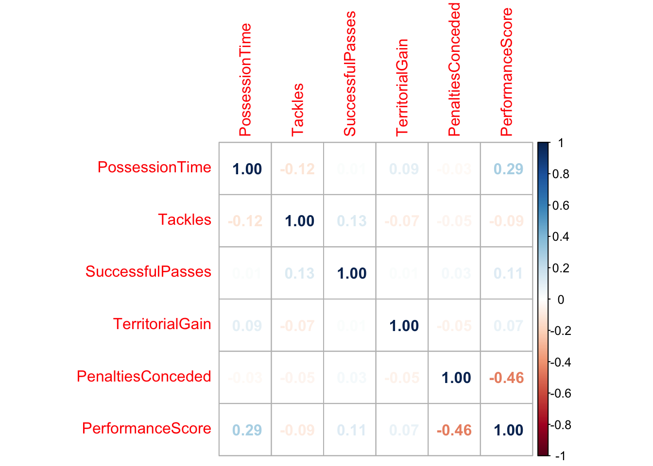
I’m going to use the a correlation matrix to explore the relationships within the data:
library(corrplot)
corrplot 0.92 loaded
cor_matrix <-cor(df) # create the correlation matrixcov_matrix <-cov(df) # create the covariance matrix# Visualise correlation matrixcorrplot(cor_matrix, method ="number")
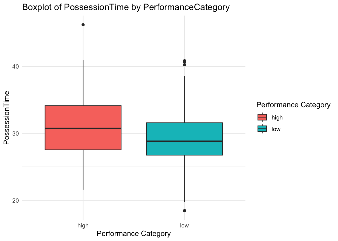
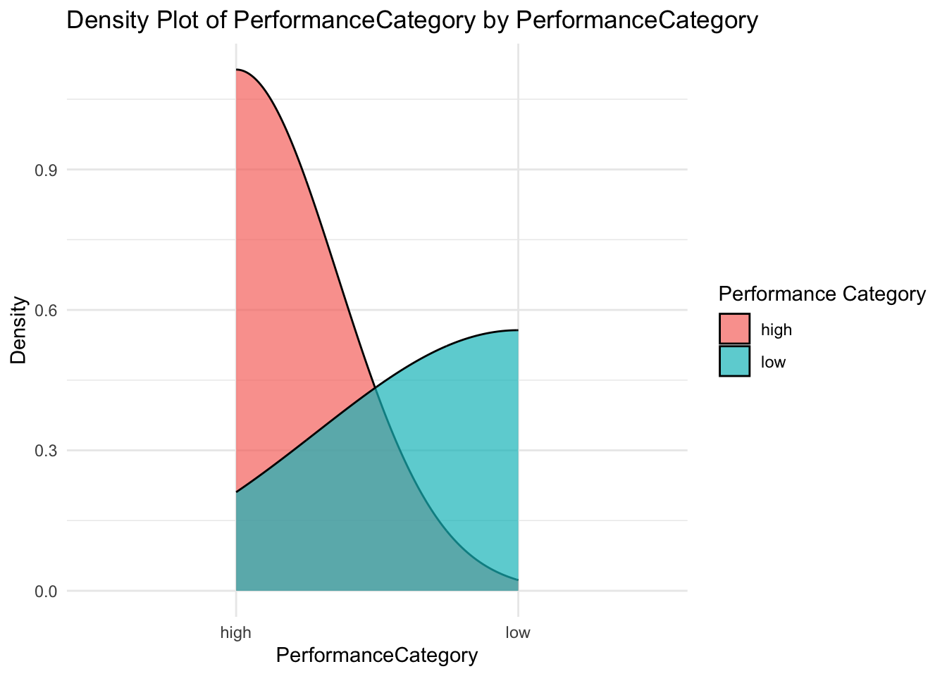
I’ll create a new variable PerformanceCategory based on how the game was scored. This allocates ‘high’ or ‘low’, depending on the PerformanceScore variable.
# Assuming df is your dataframe and PerformanceScore is the continuous variable# Calculate the median of PerformanceScore for the thresholdmedian_score <-median(df$PerformanceScore)# Create a new variable based on PerformanceScore being high or lowdf$PerformanceCategory <-ifelse(df$PerformanceScore > median_score, 'high', 'low')# Check the first few rows to verify the new variablehead(df)
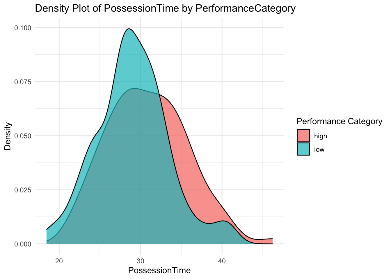
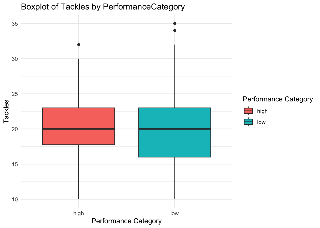
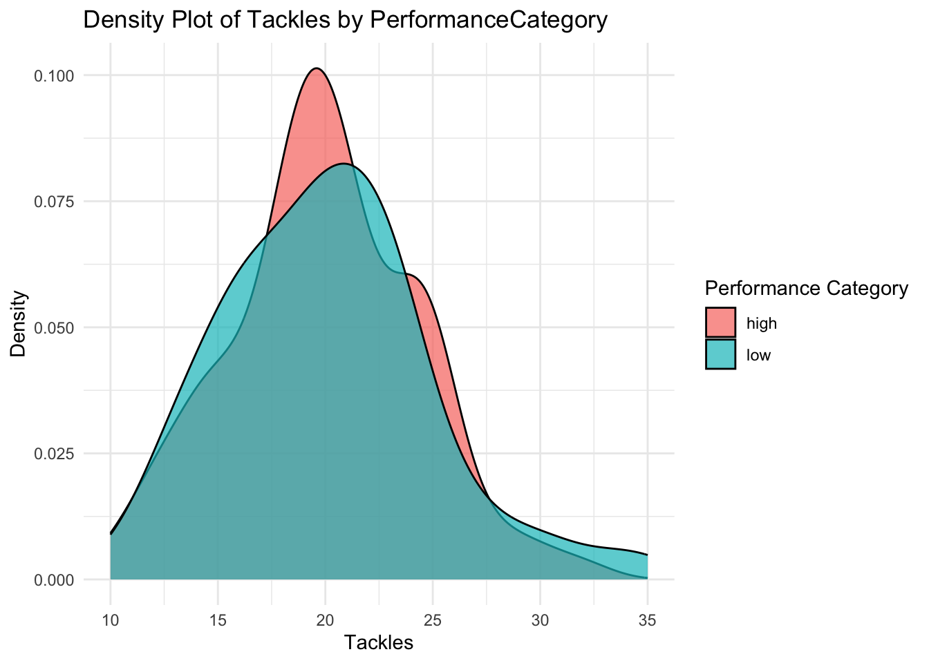
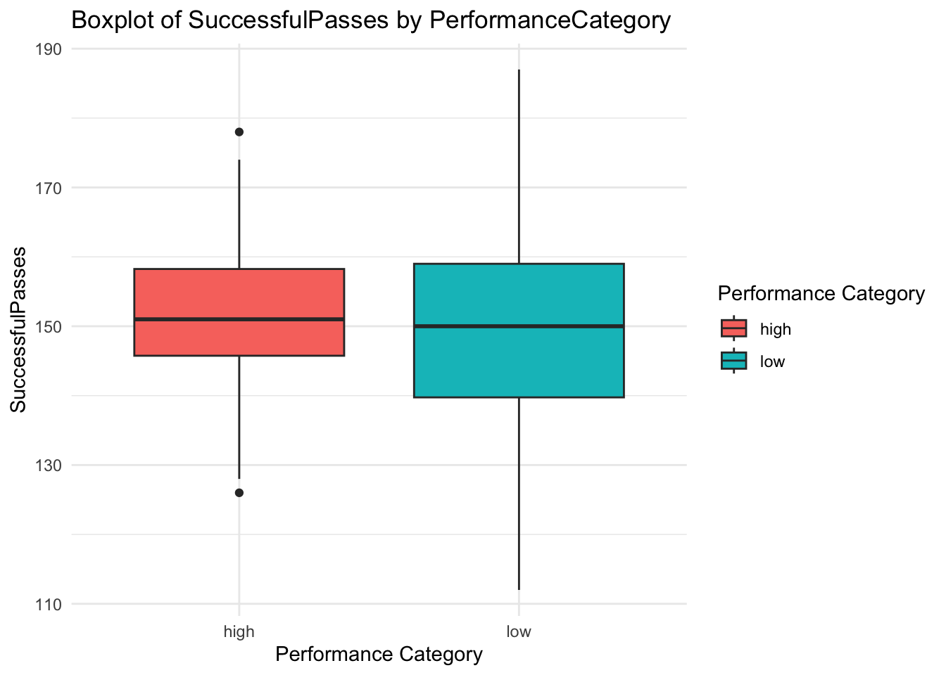
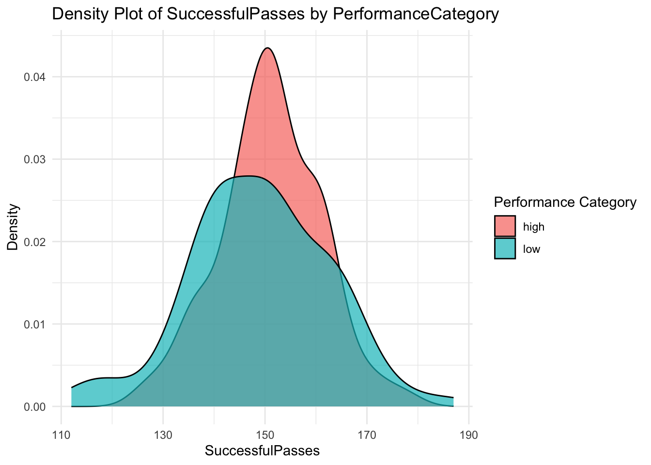
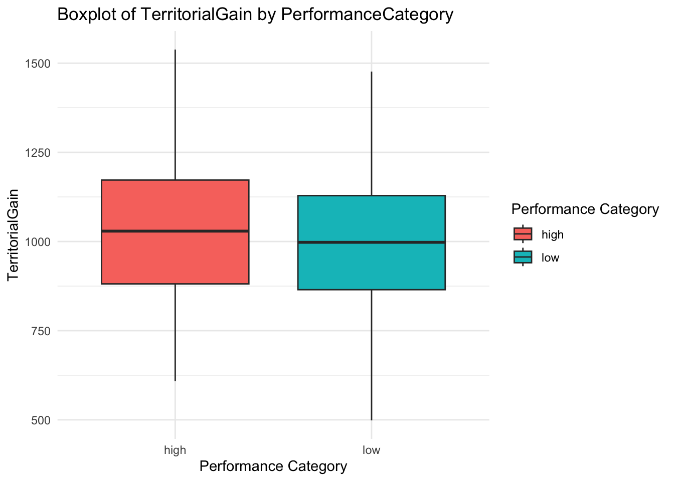
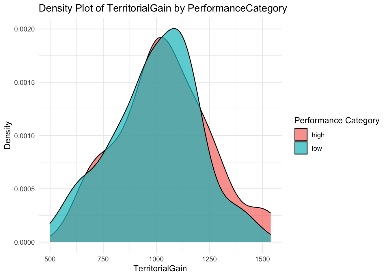
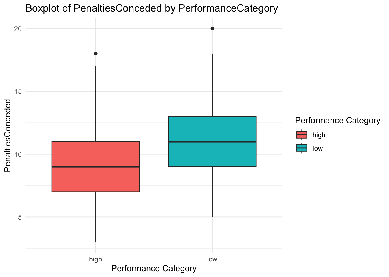
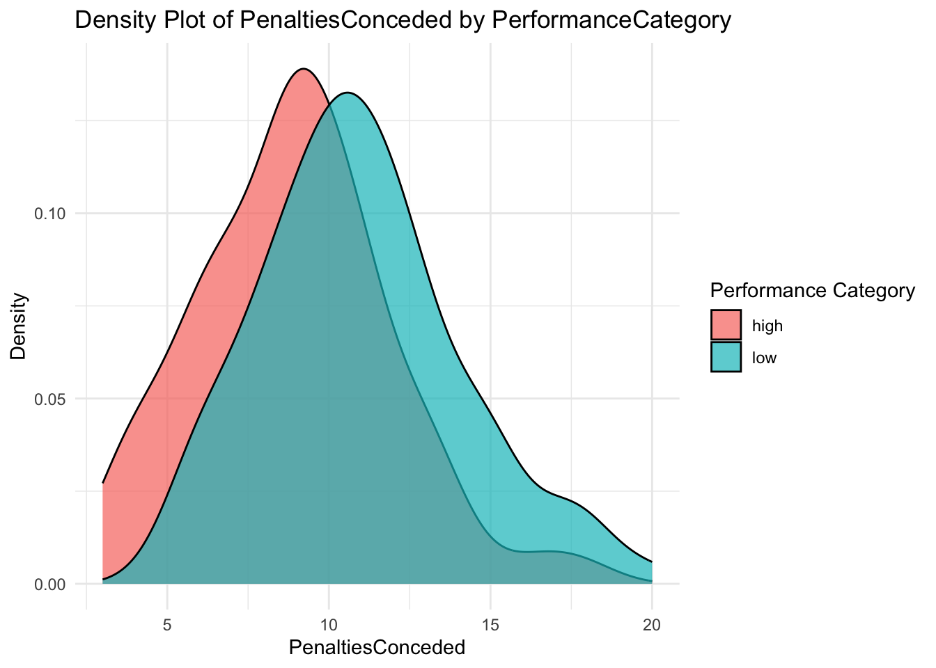
As we now have our DV in a binary variable (high or low), we can utilise boxplots and density plots to examine the apparent impact of each IV on the outcome.
# Load necessary librarieslibrary(ggplot2)library(dplyr)# Creating a list to store plotsplots_list <-list()# Iterate over each independent variable to create plotsfor (var innames(df)[-6]) { # Excluding the PerformanceCategory variable# Boxplot boxplot <-ggplot(df, aes_string(x="factor(PerformanceCategory)", y=var, fill="factor(PerformanceCategory)")) +geom_boxplot() +labs(title=paste("Boxplot of", var, "by PerformanceCategory"),x="Performance Category",y=var,fill="Performance Category") +theme_minimal()# Density plot density_plot <-ggplot(df, aes_string(x=var, fill="factor(PerformanceCategory)")) +geom_density(alpha=0.7) +labs(title=paste("Density Plot of", var, "by PerformanceCategory"),x=var,y="Density",fill="Performance Category") +theme_minimal()# Store plots in the list plots_list[[paste("Boxplot", var)]] <- boxplot plots_list[[paste("Density", var)]] <- density_plot}
Warning: `aes_string()` was deprecated in ggplot2 3.0.0.
ℹ Please use tidy evaluation idioms with `aes()`.
ℹ See also `vignette("ggplot2-in-packages")` for more information.
# Print the plotsfor (plot_name innames(plots_list)) {print(plots_list[[plot_name]])}
rm(boxplot, density_plot, plots_list)
Notice that there are some interesting associations here.
38.2.3 Step Three: Conducting the Path Analysis
We can now move on to the Path Analysis. We’re going to use the package lavaan, which is an R package designed for Path Analysis and SEM.
In the code, I’m going to specify a simple model in which all the IVs directly predict the DV. There are no mediating variables hypothesised in the model.
library(lavaan)# Define our path analysis modelmodel <-' PerformanceScore ~ PossessionTime + Tackles + SuccessfulPasses + TerritorialGain + PenaltiesConceded'# Fit modelfit <-sem(model, data=df, estimator="MLR") # Using Maximum Likelihood estimation for robust estimation# Summarise resultssummary(fit, standardized =TRUE, fit.measures =TRUE)
lavaan 0.6.17 ended normally after 1 iteration
Estimator ML
Optimization method NLMINB
Number of model parameters 6
Number of observations 200
Model Test User Model:
Standard Scaled
Test Statistic 0.000 0.000
Degrees of freedom 0 0
Model Test Baseline Model:
Test statistic 74.414 77.298
Degrees of freedom 5 5
P-value 0.000 0.000
Scaling correction factor 0.963
User Model versus Baseline Model:
Comparative Fit Index (CFI) 1.000 1.000
Tucker-Lewis Index (TLI) 1.000 1.000
Robust Comparative Fit Index (CFI) NA
Robust Tucker-Lewis Index (TLI) NA
Loglikelihood and Information Criteria:
Loglikelihood user model (H0) -588.936 -588.936
Loglikelihood unrestricted model (H1) -588.936 -588.936
Akaike (AIC) 1189.872 1189.872
Bayesian (BIC) 1209.662 1209.662
Sample-size adjusted Bayesian (SABIC) 1190.653 1190.653
Root Mean Square Error of Approximation:
RMSEA 0.000 NA
90 Percent confidence interval - lower 0.000 NA
90 Percent confidence interval - upper 0.000 NA
P-value H_0: RMSEA <= 0.050 NA NA
P-value H_0: RMSEA >= 0.080 NA NA
Robust RMSEA 0.000
90 Percent confidence interval - lower 0.000
90 Percent confidence interval - upper 0.000
P-value H_0: Robust RMSEA <= 0.050 NA
P-value H_0: Robust RMSEA >= 0.080 NA
Standardized Root Mean Square Residual:
SRMR 0.000 0.000
Parameter Estimates:
Standard errors Sandwich
Information bread Observed
Observed information based on Hessian
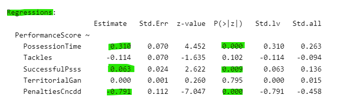
Regressions:
Estimate Std.Err z-value P(>|z|) Std.lv Std.all
PerformanceScore ~
PossessionTime 0.310 0.070 4.452 0.000 0.310 0.263
Tackles -0.114 0.070 -1.635 0.102 -0.114 -0.094
SuccessfulPsss 0.063 0.024 2.622 0.009 0.063 0.136
TerritorialGan 0.000 0.001 0.260 0.795 0.000 0.015
PenaltiesCncdd -0.791 0.112 -7.047 0.000 -0.791 -0.458
Variances:
Estimate Std.Err z-value P(>|z|) Std.lv Std.all
.PerformanceScr 21.147 2.054 10.297 0.000 21.147 0.689
38.2.4 Step Four: Interpreting the Model
There is a lot of information here! I’ll focus on the key aspects.
At the bottom, you can see a table of path coefficients (‘Regressions’):
Coefficients (‘Estimate’): These are the estimated values that show the strength and direction of the relationships between variables. A positive coefficient indicates a positive relationship, while a negative coefficient indicates a negative relationship.
Significance (‘P(>|z|)’): Look at the p-values associated with each path coefficient. A p-value less than a conventional threshold (usually 0.05) indicates that the path coefficient is statistically significant. For our current analysis, the key thing to note is the significance of ALL the IVs on the match outcome.
StandardErrors (‘Std.Err’): These provide an estimate of the variability in the path coefficients and are useful for understanding the precision of the estimates.
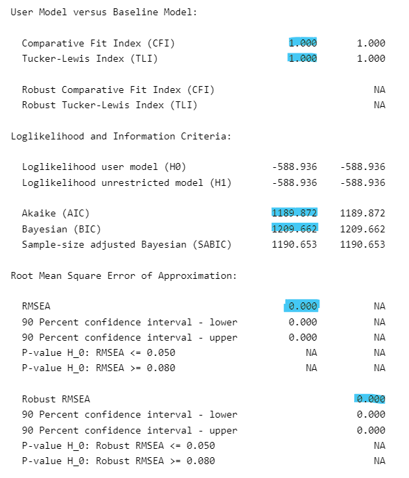
Above that table, you will see various statistics that report model fit. These let us evaluate how well the model fits the data.
Comparative Fit Index (CFI): Values above 0.90 or 0.95 suggest a goodfit.
Tucker-Lewis Index (TLI): Like the CFI, values above 0.90 or 0.95 are typically considered indicative of a goodfit.
Root Mean Square Error of Approximation (RMSEA): Values less than 0.05 indicate a close fit, and values up to 0.08 represent a reasonable error of approximation.
Standardized Root Mean Square Residual (SRMR): Values less than 0.08 are generally considered good.
38.2.4.1 Goodness of Fit Indices (AIC and BIC)
The output also provides two fit indices, which help in assessing the model fit from different perspectives. They are not particularly useful by themselves, but they help you to compare different models.
They lie outside the scope of this practical, but a general rule of thumb is that ‘lower is better’. In other words, a lower AIC for Model 2 compared with Model 1 suggests that Model 2 is ‘better’ at explaining the data, compared with Model 1.
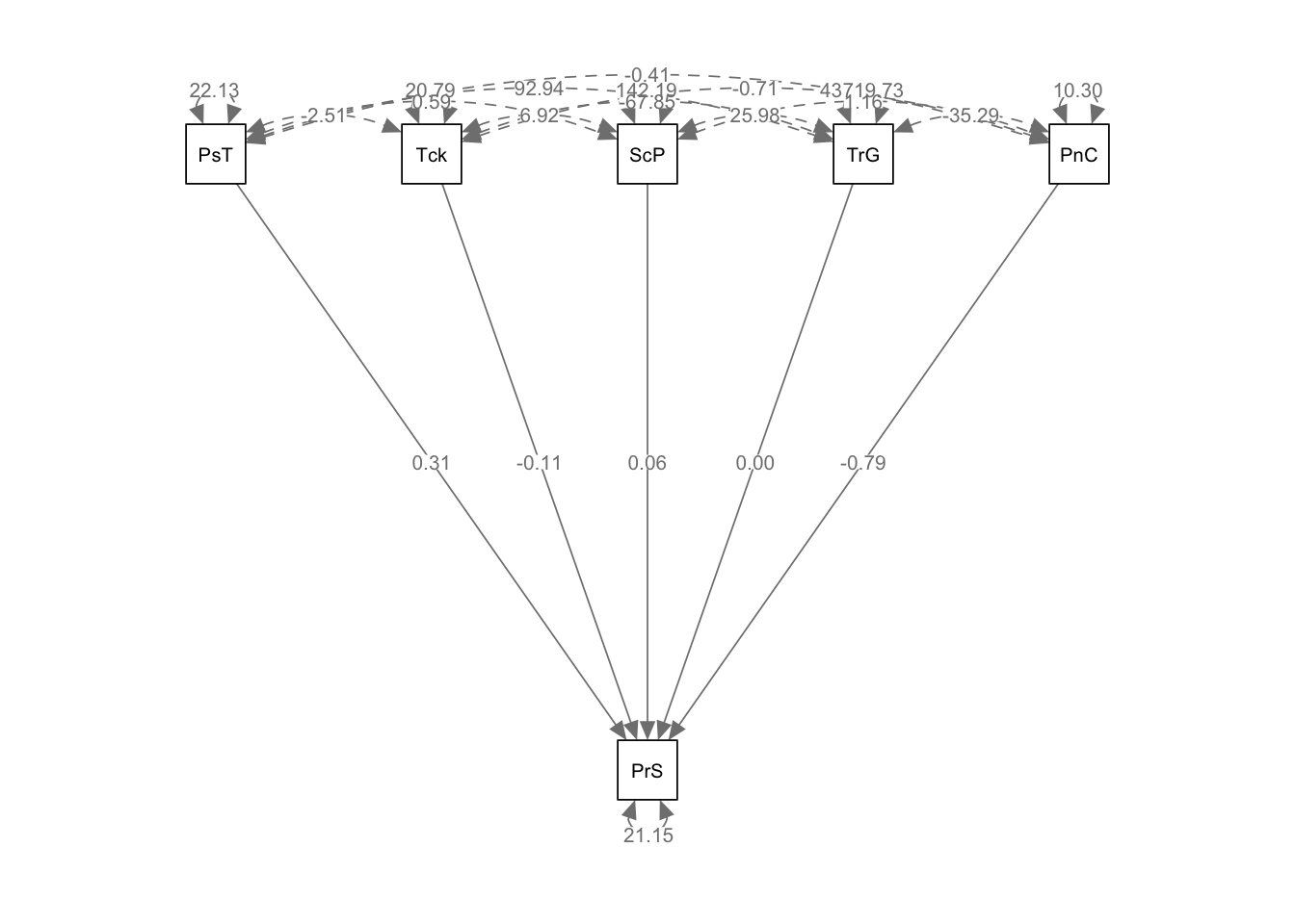
38.2.5 Step Five: Visualising the Model
We can produce a visual representation of our model using the semPlot library. I’ve
We have created a path model where PerformanceScore is regressed on all other variables (PossessionTime, Tackles, SuccessfulPasses, TerritorialGain, PenaltiesConceded).
The sem() function from the lavaan package is used to fit the model.
The `semPaths() function from the semPlot package creates a visual representation of the fitted model.
The semPlot library offers a variety of options to customize the appearance of the path diagram. For example, `whatLabels can be set to “est” to display path coefficients, “std” for standardized coefficients, or “both” for both. The layout and rotation parameters control the arrangement and orientation of the path diagram.
38.3 Path Analysis: Practice
Replicate all of the steps above on the dataset available here:
rm(list=ls())swimming_data <-read.csv('https://www.dropbox.com/scl/fi/kmzsi84wltvr9hycwnr3z/31_02.csv?rlkey=7bml7ukawcygwotuy6aemy4fr&dl=1')swimming_data$X <-NULLhead(swimming_data) # display the first six rows
The more straightforward is to conduct an analysis that assumes a direct relationship between several IVs and one DV. This is similar to the previous example. For example, you may wish to model the influence of some or all of the variables on the independent variable average speed.
Make sure to conduct EDA first, then create the statistical model, then produce a visual output of your analysis.
A more complex option is to explore the possibility of a mediating variable within the data. For example, in your hypothesis, stamina may thought to be a mediating variable on performance that is influenced by the other IVs.
If you carry out both analyses, what do you notice about the AIC? Is the mediating model a better fit with the data than the one that only models direct effects?
If you are interested in exploring path analysis further, you may wish to investigate how to include both the mediating and direct effects of variables.
Show solution for mediating variable
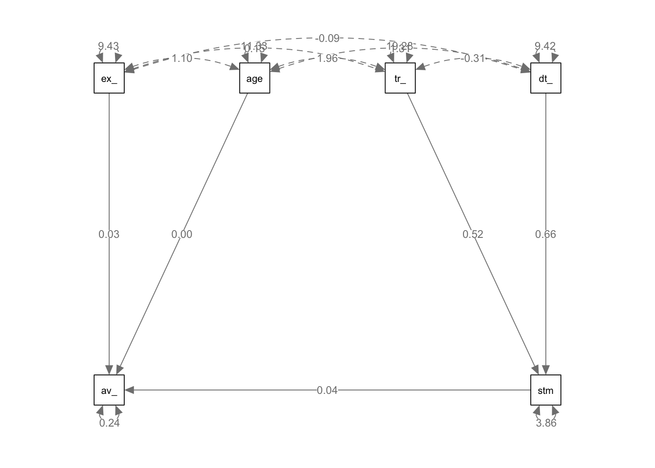
# Load lavaan packagelibrary(lavaan)# Define the model (specifying the paths)model <-' # Direct paths average_speed ~ experience_years + age + stamina # Mediation paths stamina ~ training_hours + diet_quality'# Fit modelfit <-sem(model, data = swimming_data)# Summarise resultssummary(fit, standardized =TRUE, fit.measures =TRUE)
lavaan 0.6.17 ended normally after 1 iteration

  Estimator                                         ML
  Optimization method                           NLMINB
  Number of model parameters                         7

  Number of observations                           100

Model Test User Model:

  Test statistic                                 3.820
  Degrees of freedom                                 4
  P-value (Chi-square)                           0.431

Model Test Baseline Model:

  Test statistic                               135.150
  Degrees of freedom                                 9
  P-value                                        0.000

User Model versus Baseline Model:

  Comparative Fit Index (CFI)                    1.000
  Tucker-Lewis Index (TLI)                       1.003

Loglikelihood and Information Criteria:

  Loglikelihood user model (H0)               -279.783
  Loglikelihood unrestricted model (H1)       -277.873

  Akaike (AIC)                                 573.567
  Bayesian (BIC)                               591.803
  Sample-size adjusted Bayesian (SABIC)        569.695

Root Mean Square Error of Approximation:

  RMSEA                                          0.000
  90 Percent confidence interval - lower         0.000
  90 Percent confidence interval - upper         0.148
  P-value H_0: RMSEA <= 0.050                    0.554
  P-value H_0: RMSEA >= 0.080                    0.298

Standardized Root Mean Square Residual:

  SRMR                                           0.039

Parameter Estimates:

  Standard errors                             Standard
  Information                                 Expected
  Information saturated (h1) model          Structured

Regressions:
                   Estimate  Std.Err  z-value  P(>|z|)   Std.lv  Std.all
  average_speed ~
    experience_yrs    0.030    0.016    1.879    0.060    0.030    0.180
    age               0.001    0.015    0.076    0.939    0.001    0.007
    stamina           0.035    0.014    2.574    0.010    0.035    0.248
  stamina ~
    training_hours    0.522    0.045   11.663    0.000    0.522    0.635
    diet_quality      0.662    0.064   10.331    0.000    0.662    0.563

Variances:
                   Estimate  Std.Err  z-value  P(>|z|)   Std.lv  Std.all
   .average_speed     0.239    0.034    7.071    0.000    0.239    0.905
   .stamina           3.864    0.546    7.071    0.000    3.864    0.297
We use Structural Equation Modeling (SEM) when we suspect there may be underlying (‘latent’) variables present in our data, similar to the concept introduced in our section on Factor Analysis.
SEM lets us explore this kind of complex model using a combination of factor analysis and regression.
As with everything we’re covering, this is just intended to be a basic introduction to the topic!
38.4.1 Step One: Load data
Show code for data creation
rm(list=ls())set.seed(123) # Ensure reproducibility# Number of observationsn <-500# Simulating independent variablesplayer_age <-round(rnorm(n, 25, 4),0) # Player age in yearsyears_in_NFL <-round(rnorm(n, 3, 2),0) # Years in NFLgames_played <-round(rpois(n, 16),0) # Games played in a seasontotal_yards <-round(rnorm(n, 500, 150),0) # Total yardstouchdowns <-round(rpois(n, 5),0) # Touchdownsinterceptions <-round(rpois(n, 2),0) # Interceptionstackles <-rpois(n, 40) # Tackles madesacks <-rpois(n, 5) # Sacks# Simulating latent variables "Performance" and "Experience"# For simulation purposes, we will create proxies for these latent constructs.performance_proxy <- total_yards + touchdowns*10- interceptions*5+ tackles + sacks*2experience_proxy <- player_age + years_in_NFL*2# Normalise proxies to have them on a similar scaleperformance_proxy <-scale(performance_proxy)experience_proxy <-scale(experience_proxy)# Simulating "Player Value" influenced by "Performance" and "Experience"player_value <-round(5*performance_proxy +3*experience_proxy +rnorm(n, 0, 1),2) # Add noise# Create dataframedata <-data.frame(player_age, years_in_NFL, games_played, total_yards, touchdowns, interceptions, tackles, sacks, player_value)# View the first few rows of the datasethead(data)
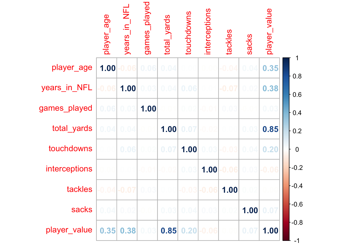
# Load necessary librarieslibrary(dplyr)library(ggplot2)library(lavaan)# Exploratory Data Analysislibrary(corrplot)cor_matrix <-cor(data) # create the correlation matrixcov_matrix <-cov(data) # create the covariance matrix# Visualise correlation matrixcorrplot(cor_matrix, method ="number")
rm(cor_matrix, cov_matrix)
38.4.3 Step Three: Specify the Structural Equation Model (SEM)
As for path analysis, we need to define the model.
The independent variable we are investigating is player_value. We could create a path analysis that looks at direct relationships between these variables.
Unlike path analysis, which only deals with observed variables, in SEM model-building involves specifying any hypothesised latent variables, and the relationships among them.
Remember: that’s the reason we use SEM rather than path analysis.
For simplicity, let’s assume a model where Performance is a latent variable indicated by total_yards and touchdowns, while a second latent variable is called Experience and is indicated by player_age and years_in_NFL.
I’ll use the lavaan package to estimate the model.
Before doing so, I’m going to standardise my variables, which can be helpful if different variables are measured on very different scales.
# Scale the variablesdata$player_age <-scale(data$player_age)data$years_in_NFL <-scale(data$years_in_NFL)data$games_played <-scale(data$games_played)data$total_yards <-scale(data$total_yards)data$touchdowns <-scale(data$touchdowns)data$interceptions <-scale(data$interceptions)data$tackles <-scale(data$tackles)data$sacks <-scale(data$sacks)data$player_value <-scale(data$player_value)# Fit the modelfit <-sem(model, data = data, estimator ="MLR", control =list(maxit =15000)) # Increase max iterations to 10000# Model summarysummary(fit, fit.measures =TRUE)
lavaan 0.6.17 ended normally after 1169 iterations
Estimator ML
Optimization method NLMINB
Number of model parameters 12
Number of observations 500
Model Test User Model:
Standard Scaled
Test Statistic 1.438 1.587
Degrees of freedom 3 3
P-value (Chi-square) 0.697 0.662
Scaling correction factor 0.906
Yuan-Bentler correction (Mplus variant)
Model Test Baseline Model:
Test statistic 1763.412 1856.167
Degrees of freedom 10 10
P-value 0.000 0.000
Scaling correction factor 0.950
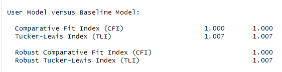
User Model versus Baseline Model:
Comparative Fit Index (CFI) 1.000 1.000
Tucker-Lewis Index (TLI) 1.003 1.003
Robust Comparative Fit Index (CFI) 1.000
Robust Tucker-Lewis Index (TLI) 1.002
Loglikelihood and Information Criteria:
Loglikelihood user model (H0) -2663.857 -2663.857
Scaling correction factor 1.033
for the MLR correction
Loglikelihood unrestricted model (H1) -2663.138 -2663.138
Scaling correction factor 1.007
for the MLR correction
Akaike (AIC) 5351.714 5351.714
Bayesian (BIC) 5402.289 5402.289
Sample-size adjusted Bayesian (SABIC) 5364.200 5364.200
Root Mean Square Error of Approximation:
RMSEA 0.000 0.000
90 Percent confidence interval - lower 0.000 0.000
90 Percent confidence interval - upper 0.056 0.062
P-value H_0: RMSEA <= 0.050 0.926 0.899
P-value H_0: RMSEA >= 0.080 0.008 0.013
Robust RMSEA 0.000
90 Percent confidence interval - lower 0.000
90 Percent confidence interval - upper 0.056
P-value H_0: Robust RMSEA <= 0.050 0.926
P-value H_0: Robust RMSEA >= 0.080 0.006
Standardized Root Mean Square Residual:
SRMR 0.014 0.014
Parameter Estimates:
Standard errors Sandwich
Information bread Observed
Observed information based on Hessian
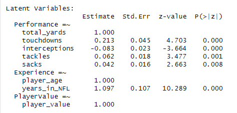
Latent Variables:
Estimate Std.Err z-value P(>|z|)
Performance =~
total_yards 1.000
touchdowns 0.216 0.048 4.523 0.000
Experience =~
player_age 1.000
years_in_NFL 1.092 0.108 10.081 0.000
PlayerValue =~
player_value 1.000
Regressions:
Estimate Std.Err z-value P(>|z|)
PlayerValue ~
Performance 3.038 1.210 2.512 0.012
Experience -4.406 3.605 -1.222 0.222
Covariances:
Estimate Std.Err z-value P(>|z|)
Performance ~~
Experience 0.041 0.028 1.448 0.148
Variances:
Estimate Std.Err z-value P(>|z|)
.total_yards 0.660 0.144 4.577 0.000
.touchdowns 0.982 0.078 12.527 0.000
.player_age 1.050 0.075 13.920 0.000
.years_in_NFL 1.060 0.083 12.788 0.000
.player_value 0.000
Performance 0.338 0.139 2.437 0.015
Experience -0.052 0.040 -1.290 0.197
.PlayerValue -0.025 1.594 -0.016 0.987
38.4.5 Step Five: Inspect the model
Interpreting the outputs from a structural equation model (SEM) using the lavaan package in R involves understanding various components of the model output. Here’s a guide to some of the key elements you’ll find in the output:
Model Estimation Summary Estimates: This section shows the estimated parameters of the model. In SEM, these include factor loadings (relationships between observed variables and latent variables), regression weights (relationships among latent variables), and variances and covariances of the variables.
Factor Loadings: Indicate how strongly each observed variable represents the latent variable. Higher absolute values indicate a stronger relationship.
Regression Weights: Show the direction and strength of the relationships between latent variables.
Significance: Usually indicated by p-values. A p-value less than 0.05 typically suggests that the parameter is significantly different from zero, lending support to that part of the model.
Fit Indices The output provides various fit indices which help in evaluating how well the model fits the data. Common indices include:
Chi-Square Test of Model Fit (χ²): A non-significant chi-square (p > 0.05) suggests a good fit. However, it’s sensitive to sample size.
Comparative Fit Index (CFI): Values closer to 1 indicate a good fit, with values above 0.90 or 0.95 often considered indicative of a good fit.
Tucker-Lewis Index (TLI): Similar to CFI, with values close to 1 suggesting a good fit. Values above 0.90 are typically considered good.
Root Mean Square Error of Approximation (RMSEA): Values less than 0.05 indicate a close fit, values up to 0.08 represent a reasonable error of approximation, and values greater than 0.10 suggest a poor fit.
Standardized Root Mean Square Residual (SRMR): Represents the difference between the observed correlation and the model-predicted correlation. Values less than 0.08 are generally considered good.
38.4.6 Step Six: Evaluate Model Fit
Check various fit indices like CFI, TLI, RMSEA to evaluate the model.
Comparative Fit Index (CFI): Values above 0.90 or 0.95 suggest a goodfit.
Tucker-Lewis Index (TLI): Like the CFI, values above 0.90 or 0.95 are typically considered indicative of a goodfit.
Root Mean Square Error of Approximation (RMSEA): Values less than 0.05 indicate a close fit, and values up to 0.08 represent a reasonable error of approximation.
Standardized Root Mean Square Residual (SRMR): Values less than 0.08 are generally considered good.
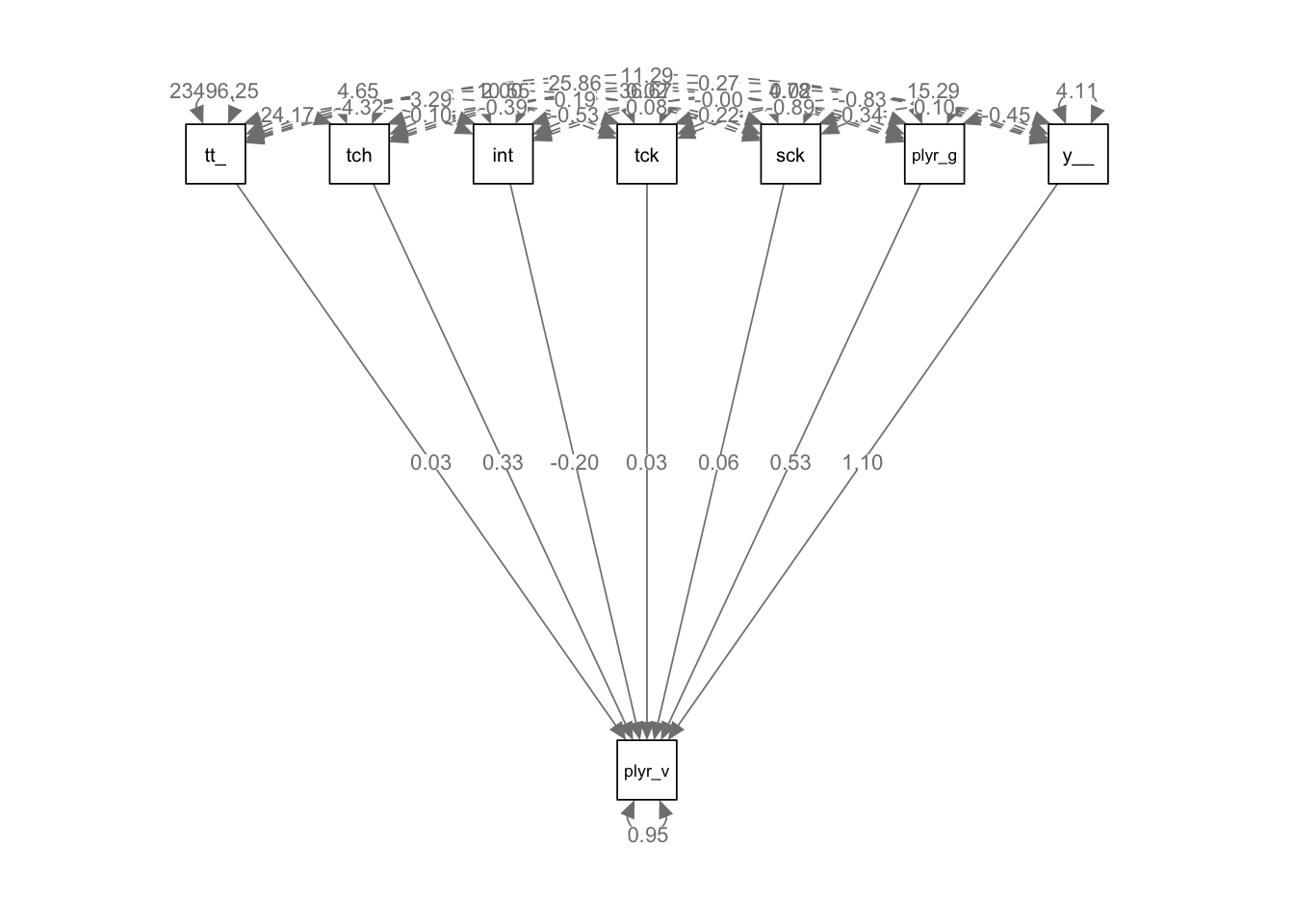
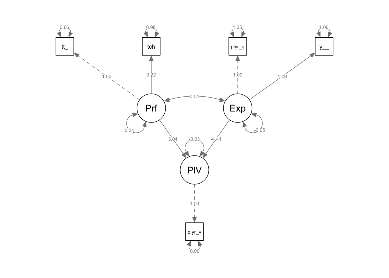
We can use the semPlot package for visual representation.
library(semPlot)# SEM plotsemPaths(fit, whatLabels ="est", layout ="tree")
38.5 SEM: Practice
Repeat the process from the demonstration.
This time, build an alternative model (for example, where Experience is influenced by player value, years in NFL, and Performance is by tackles and sacks) . You could use touchdowns as your Independent Variable.